Valve manual
Valve application is a driver that uses aquaduct module to perform analysis of trajectories of selected residues in Molecular Dynamics simulation.
Valve invocation
Once aquaduct module is installed (see Aqua-Duct installation guide) properly on the machine, Valve is available as valve.py command line tool.
Usage
Basic help of Valve usage can be displayed by the following command:
valve.py --help
It should display the following information:
usage: valve.py [-h] [-c CONFIG_FILE] [-t THREADS] [--force-save] [--debug]
                [--debug-file DEBUG_FILE] [--version] [--license]
                [--dump-template-config]

Valve, Aquaduct driver

optional arguments:
  -h, --help            show this help message and exit
  -c CONFIG_FILE        Config file filename. (default: None)
  -t THREADS            Limit Aqua-Duct calculations to given number of
                        threads. (default: None)
  --force-save          Force saving results. (default: False)
  --debug               Prints debug info. (default: False)
  --debug-file DEBUG_FILE
                        Debug log file. (default: None)
  --version             Prints versions and exits. (default: False)
  --license             Prints short license info and exits. (default: False)
  --dump-template-config
                        Dumps template config file. Suppress all other output
                        or actions. (default: False)
Configuration file template
Configuration file used by Valve is of moderate length and complexity. It can be easily prepared with a template file that can be printed by Valve. Use the following command to print configuration file template on the screen:
valve.py --dump-template-config
Configuration file template can also be easily saved as a file with:
valve.py --dump-template-config > config.txt
Where config.txt is a configuration file template.
For detailed description of configuration file and available options see Configuration file options.
Valve calculation run
Once configuration file is ready Valve calculations can be run with the following simple command:
valve.py -c config.txt
Some of Valve calculations can be run in parallel. By default all available CPU cores are used. This is not always desired - limitation of used CPU cores can be done with -t option which limits number of concurrent threads used by Valve. If it equals 1 no parallelism is used.
Note
Specifying number of threads greater than the available CPU cores is generally not optimal.
However, in order to maximize the usage of available CPU power it is recommended to set it as the actual number of cores + 1. It is caused by the fact that Valve uses one thread for the main process and the more than one threads for processes of parallel calculations. When parallel calculations are executed the main thread waits for results.
Debugging
Valve can output some debug information. Use --debug to see all debug information on the screen or use --debug-file with some file name to dump all debug messages to the given file. Beside debug messages, standard messages will be saved in the file as well.
How does Valve work
Application starts with parsing input options. If --help or --dump-template-config options are used, appropriate messages are printed on the screen and Valve quits with signal 0.
Note
In current version Valve does not check the validity of the config file.
If config file is provided (option -c) Valve parses it quickly and regular calculations start according to their contents. Calculations performed by Valve are done in six stages which are described in the next sections.
Traceable residues
In the first stage of calculations Valve finds all residues that should be traced and appends them to the list of traceable residues. It is done in a loop over all frames. In each frame residues of interest are searched and appended to the list but only proveded that they are not already present on the list. In sandwich mode this is repeated for each layer.
The search of traceable residues is done according to specifications provided by user. Two requirements have to be met to append residue to the list:
The residue has to be found according to the object definition.
The residue has to be within the scope of interest.
The object definition usually encompasses the active site of the protein (or other region of interest of macromolecule in question). The scope of interest defines, on the other hand, the boundaries in which residues are traced and is usually defined as protein.
Since aquaduct, in its current version, uses MDAnalysis Python module for reading, parsing and searching of MD trajectory data, definitions of object and scope have to be given as its Selection Commands.
Object definition
Object definition has to comprise of two elements:
It has to define residues to trace.
It has to define spatial boundaries of the object site.
For example, proper object definition could be as following:
(resname WAT) and (sphzone 6.0 (resnum 99 or resnum 147))
It defines WAT as residues that should be traced and defines spatial constrains of the object site as spherical zone within 6 Angstroms from the center of masses of residues with number 99 and 147.
Scope definition
Scope can be defined in two ways: as object but with broader boundaries or as the convex hull of selected molecular object.
In the first case definition is very similar to object and it has to follow the same limitations. For example, a proper scope definition could be as follows:
resname WAT and around 2.0 protein
It consequently has to define WAT as residues of interest and defines spatial constrains: all WAT residues that are within 2 Angstroms of the protein.
If the scope is defined as the convex hull of selected molecular object (which is recommended), the definition itself has to comprise of this molecular object only, for example protein. In that case the scope is interpreted as the interior of the convex hull of atoms from the definition. Therefore, traceable residues would be in the scope only if they were within the convex hull of atoms of protein.
Convex hulls of macromolecule atoms
AQ uses quickhull algorithm for convex hull calculations (via SciPy class scipy.spatial.ConvexHull, see also http://www.qhull.org/ and original publication The quickhull algorithm for convex hulls).
Convex hull concept is used to check if traced molecules are inside of the macromolecule. Convex hull can be considered as rough approximation of molecular surface. The following picture shows schematic comparison of convex hull and solvent excluded surface (SES):
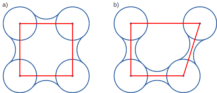
Convex hull (red shape) of atoms (blue dots with VdW spheres) and SES (blue line): a) convex hull and SES cover roughly the same area, convex hull approximates SES; b) movement of one atom dramatically changes SES, however, interior of the molecule as approximated by convex hull remains stable.
No doubts, convex hull is a very rough approximation of SES. It has, however, one very important property when it is used to approximate interior of molecules: its interior does not considerably depend on the molecular conformation of a molecule (or molecular entity) in question.
Convex hull inflation
AQ allows to alter size of the scope convex hulls by means of inflate options. Once scope is defined as convex hull of particular atoms, vertices of it can be interpreted as vectors originating in the center of geometry of the convex hull. Value of inflate option is added to such vectors and in consequence theirs leghts are increased (or decreased if added value is negative). Finally, convex hull is recalculated using points resulting from inflated vectors.
In reference to the previous picture, consider the following example:
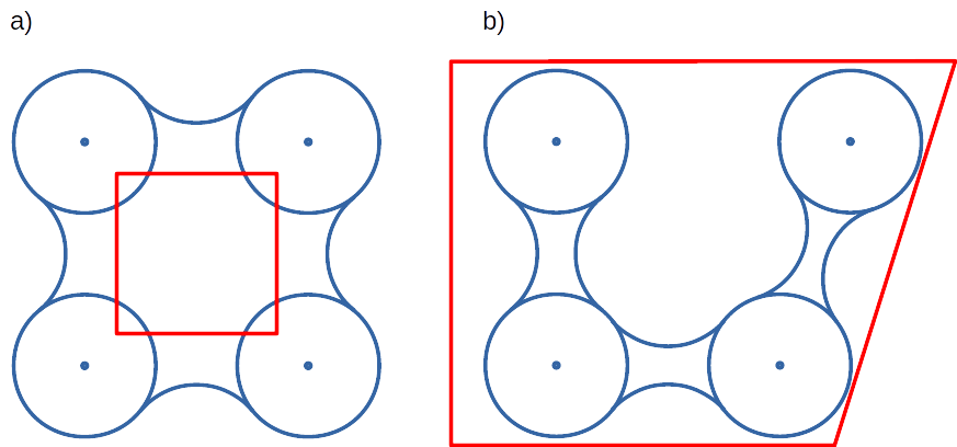
On the left panel a) convex hull was deflated with negative value of inflate option, whareas on the right panel b) convex hull was inflated with positive value of inflate option.
This feautre is available in all stages where scope convex hull is used. For more details on configuration look for inflate options in the configuration file.
Raw paths
The second stage of calculations uses the list of all traceable residues from the first stage and for every residue in each frame two checks are performed:
Is the residue in the scope (this is always calculated according to the scope definition).
Is the residue in the object. This information is partially calculated in the first stage and can be reused in the second. However, it is also possible to recalculate this data according to the new object definition.
For each of the traceable residues a special Path object is created which stores frames in which a residue is in the scope or in the object.
Note
Residue is in the object only if it is also in the scope.
Separate paths
The third stage uses collection of Path objects to create Separate Path objects. Each Path comprises data for one residue. It may happen that the residue enters and leaves the scope and the object many times over the entire MD. Each such event is considered by Valve as a separate path.
There are two types of Separate Paths:
Object Paths
Passing Paths
Object Paths are traces of molecules that visited Object area. Passing Paths are traces of molecules that entered Scope but did not entered Object area.
Passing paths comprises of one part only. Each object path comprises of following parts:
Incoming - Defined as a path that leads from the point in which residue enters the scope and enters the object for the first time.
Object - Defined as a path that leads from the point in which residue enters the object for the first time and leaves it for the last time.
[Optional] Out of active site - Defined as a path between the Object paths that leads from the point in which residue leaves the object but stays within the scope and enters the object again.
Outgoing - Defined as a path that leads from the point in which residue leaves the object for the last time and leaves the scope.
It is also possible that incoming and/or outgoing part of the separate path is empty.
Note
Generation of Passing paths is optional and can be switched off.
Warning
Generation of Passing paths without redefinition of Object area in stage I and II may lead to false results.
Auto Barber
After the initial search of Separate Path objects, it is possible to run Auto Barber procedure which trims paths down to the approximated surface of the macromolecule or other molecular entity defined by the user. This trimming is done by creating collection of spheres that have centers at the ends of paths and radii equal to the distance from the center to the nearest atom of user defined molecular entity. Next, parts of raw paths that are inside these spheres are removed and separate paths are recreated.
Auto Barber procedure has several options, for example:
auto_barber allows to define molecular entity which is used to calculate radii of spheres used for trimming raw paths.
auto_barber_mincut allows to define minimal radius of spheres. Spheres of radius smaller than this value are not used in trimming.
auto_barber_maxcut allows to define maximal radius of spheres. Spheres of radius greater than this value are not used in trimming.
auto_barber_tovdw if set to True radii of spheres are corrected (decreased) by Van der Waals radius of the closest atom.
See also options of separate_paths stage.
Smoothing
Separate paths can be optionally smoothed. Current aquaduct version allows to perform soft smoothing only, i.e. smoothing is used only for visualization purposes. Raw paths cannot be replaced by the smoothed.
Available methods
Aqua-Duct implements several smoothing methods:
Savitzky-Golay filter -
SavgolSmooth- see also original publication Smoothing and Differentiation of Data by Simplified Least Squares Procedures (doi:10.1021/ac60214a047).Window smoothing -
WindowSmoothDistance Window smoothing -
DistanceWindowSmoothActive Window smoothing -
ActiveWindowSmoothMax Step smoothing -
MaxStepSmoothWindow over Max Step smoothing -
WindowOverMaxStepSmoothDistance Window over Max Step smoothing -
DistanceWindowOverMaxStepSmoothActive Window over Max Step smoothing -
ActiveWindowOverMaxStepSmooth
For detailed information on available configuration options see configuration file smooth section description.
Clustering of inlets
Each of the separate paths has the beginning and end. If they are at the boundaries of the scope they are considered as Inlets, i.e. points that mark where the traceable residues enter or leave the scope. Clusters of inlets, on the other hand, mark endings of tunnels or ways in the system which were simulated in the MD.
Clustering of inlets is performed in the following steps:
Initial clustering: All inlets are submitted to selected clustering method and depending on the method and settings, some of the inlets might not be arranged to any cluster and are considered as outliers.
[Optional] Outliers detection: Arrangement of inlets to clusters is sometimes far from optimal. In this step, inlets that do not fit into cluster are detected and annotated as outliers. This step can be executed in two modes:
Automatic mode: Inlet is considered to be an outlier if its distance from the centroid is greater than the mean distance + 4 * standard deviation of all distances within the cluster.
Defined threshold: Inlet is considered to be an outlier if its minimal distance from any other point in the cluster is greater than the threshold.
[Optional] Reclustering of outliers: It may happen that the outliers form actually clusters but it was not recognized in the initial clustering. In this step clustering is executed only for outliers and the clusters that were found are appended to the clusters identified in the first step. Rest of the inlets are marked as outliers.
Potentially recursive clustering
Both Initial clustering and Reclustering can be run in a recursive manner. If in the appropriate sections defining clustering methods option recursive_clustering is used, appropriate method is run for each cluster separately. Clusters of specific size can be excluded from recursive clustering (option recursive_threshold). It is also possible to limit maximal number of recursive levels - option max_level.
For additional information see clustering sections options.
Available methods
Aqua-Duct implements several clustering methods. The recommended method is barber method which bases on Auto Barber procedure. Rest of the methods are implemented with sklearn.cluster module:
aquaduct.geom.cluster.BarberCluster- default for Initial clustering. It gives excellent results. For more information see barber clustering method description.MeanShift- see also original publication Mean shift: a robust approach toward feature space analysis (doi:10.1109/34.1000236).DBSCAN- default for Reclustering of outliers, see also original publication A Density-Based Algorithm for Discovering Clusters in Large Spatial Databases with NoiseAffinityPropagation- see also original publication Clustering by Passing Messages Between Data Points (doi:10.1126/science.1136800)KMeans- see also k-means++: The advantages of careful seeding, Arthur, David, and Sergei Vassilvitskii in Proceedings of the eighteenth annual ACM-SIAM symposium on Discrete algorithms, Society for Industrial and Applied Mathematics (2007), pages 1027-1035.Birch- see also Tian Zhang, Raghu Ramakrishnan, Maron Livny BIRCH: An efficient data clustering method for large databases and Roberto Perdisci JBirch - Java implementation of BIRCH clustering algorithm.
For additional information see clustering sections options.
Master paths
At the end of clustering stage it is possible to run procedure for master path generation. First, separate paths are grouped according to the clusters. Paths that begin and end in particular clusters are grouped together. Next, for each group a master path (i.e., average path) is generated in the following steps:
First, length of master path is determined. Lengths of each parts (incoming, object, outgoing) for each separate paths are normalized with bias towards the longest paths. These normalized lengths are then used as weights for averaging not normalized lengths. Values for all parts are summed and resulting value is the desired length of master path.
All separate paths are divided into chunks. Number of chunks is equal to the desired length of master path calculated in the previous step. Lengths of separate paths can be quite diverse, therefore, for different paths, chunks are of different lengths.
For each chunk, the averaging procedure is run:
Coordinates for all separate paths for a given chunk are collected.
Normalized lengths with bias toward the longest paths for all separate paths for a given chunk are collected.
New coordinates are calculated as weighted average of collected coordinates. Collected normalized lengths are used as weights.
In addition, width of chunk is calculated as a mean value of collected coordinates of mutual distances.
Type of chunk is calculated as probability (frequency) of being in the scope.
Results for all chunks are collected, types probability are changed to types. All data is then used to create Master Path. If this fails no path is created.
More technical details on master path generation can be found in aquaduct.geom.master.CTypeSpathsCollection.get_master_path() method documentation.
Passing paths
If Passing paths are allowed (see allow_passing_paths option in separate_paths configuration) they will be generated using list of traceable residues from the first stage of calculations. In usual settings, where Object and Scope definitions are the same in both the I and II stage, this will result in relatively low number of passing paths. In particular, this will not show the real number of traced molecules that enter the Scope during the simulation.
To get correct picture, configuration options have to be adjusted according to one of the following suggestions:
Adding passing molecules [recommended]
- Stage traceable_residues
add_passingshould define all molecules to be traced. If water is traced this should be set to e.g.resname WAT HOH TIP.
- Stage separate_paths
allow_passing_pathsshould be set toTrue. This allows generation of passing paths.
Redefinition of scope and object areas
- Stage traceable_residues
objectshould be broad enough to encompass all molecules that should be traced. For example, if water is traced,objectdefinition could be as following:resname WAT.
- Stage raw_paths
In order to retain default Aqua-Duct behavior of tracing molecules that flow through Object area, it have to be redefined to encompass the active site only - see Object definition discussion.
clear_in_object_infoshould be set toTrue. Otherwise, traceable molecules will be limited according to the currentobjectdefinition but Object boundaries from traceable_residues stage will be used.
- Stage separate_paths
allow_passing_pathsshould be set toTrue. This allows generation of passing paths.
Clustering of passing paths
Additionally, in stage inlets_clustering, the following options could also be adjusted:
exclude_passing_in_clusteringcould be set toTrue. This will exclude the passing paths inlets from clustering.If passing paths are not clustered they will be added as outliers. Option
add_passing_to_clustersallows to add some of passing paths inlets to the already existing clusters. This is done by Auto Barber method and therefore this option should define molecular entity used in Auto Barber procedure, for exampleprotein.
Analysis
Fifth stage of Valve calculations analyses results calculated in stages 1 to 4. Results of the analysis are displayed on the screen or can be saved to a text file and comprise of several parts.
General summary
Results start with a general summary.
Title and data stamp.
[Optional] Dump of configuration options.
Frames window.
- Names of traced molecules.
Note
If more than one name is on the list all consecutive sections of Analysis results are provided for each name separately, as well as for all names.
Number of traceable residues.
Number of separate paths.
Number of inlets.
- Number of clusters.
Outliers flag, yes if they are present.
Clustering history - a tree summarizing calculated clusters.
Clusters statistics
- Clusters summary - inlets.
- Summary of inlets clusters. Table with 4 columns:
Cluster: ID of the cluster. Outliers have 0.
Size: Size of the cluster.
INCOMING: Number of inlets corresponding to separate paths that enter the scope.
OUTGOING: Number of inlets corresponding to separate paths that leave the scope.
- Cluster statistics.
- Probabilities of transfers. Table with 7 columns:
Cluster: ID of the cluster. Outliers have 0.
IN-OUT: Number of separate paths that both enter and leave the scope by this cluster.
- diff: Number of separate paths that:
Enter the scope by this cluster but leave the scope by another cluster, or
Enter the scope by another cluster but leave the scope by this cluster.
- N: Number of separate paths that:
Enter the scope by this cluster and stays in the object, or
Leaves the scope by this cluster after staying in the object.
IN-OUT_prob: Probability of IN-OUT.
diff_prob: Probability of diff.
N_prob: Probability of N.
- Mean lengths of transfers. Table with 8 columns:
Cluster: ID of the cluster. Outliers have 0.
X->Obj: Mean length of separate paths leading from this cluster to the object.
Obj->X: Mean length of separate paths leading from the object to this cluster.
p-value: p-value of ttest of comparing X->Obj and Obj->X.
X->ObjMin: Minimal value of length of separate paths leading from this cluster to the object.
X->ObjMinID: ID of separate path for which X->ObjMin was calculated.
Obj->XMin: Minimal value of length of separate paths leading from the object to this cluster.
Obj->XMinID: ID of separate path for which Obj->XMin was calculated.
- Mean frames numbers of transfers. Table with 8 columns:
Cluster: ID of the cluster. Outliers have 0.
X->Obj: Mean number of frames of separate paths leading from this cluster to the object.
Obj->X: Mean number of frames of separate paths leading from the object to this cluster.
p-value: p-value of ttest of comparing X->Obj and Obj->X.
X->ObjMin: Minimal value of number of frames of separate paths leading from this cluster to the object.
X->ObjMinID: ID of separate path for which X->ObjMin was calculated.
Obj->XMin: Minimal value of number of frames of separate paths leading from the object to this cluster.
Obj->XMinID: ID of separate path for which Obj->XMin was calculated.
Note
Distributions of X->Obj and Obj->X might be not normal, ttest may result in unrealistic values. This test will be changed in the future releases.
Clusters types statistics
- Separate paths clusters types summary. Tables with 11 columns.
- Mean length of paths:
CType: Separate path Cluster Type.
Size: Number of separate paths belonging to Cluster type.
Size%: Percentage of Size relative to the total number of separate paths.
Tot: Average total length of paths.
TotStd: Standard deviation of Tot.
Inp: Average length of incoming part of paths. If no incoming parts are available, NaN is printed (not a number).
InpStd: Standard deviation of Inp.
Obj: Average length of object part of paths. If no incoming parts are available, NaN is printed.
ObjStd: Standard deviation of Inp.
Out: Average length of outgoing part of paths. If no incoming parts are available, NaN is printed.
OutStd: Standard deviation of Inp.
- Mean number of frames:
CType: Separate path Cluster Type.
Size: Number of separate paths belonging to Cluster type.
Size%: Percentage of Size relative to the total number of separate paths.
Tot: Average total number of frames of paths.
TotStd: Standard deviation of Tot.
Inp: Average total number of incoming part of paths. If no incoming parts are available, NaN is printed (not a number).
InpStd: Standard deviation of Inp.
Obj: Average total number of object part of paths. If no incoming parts are available, NaN is printed.
ObjStd: Standard deviation of Inp.
Out: Average total number of outgoing part of paths. If no incoming parts are available, NaN is printed.
OutStd: Standard deviation of Inp.
Cluster Type of separate path
Clusters types (or CType) is a mnemonic for separate paths that leads from one cluster to another, including paths that start/end in the same cluster or start/end in the Object area.
Each separate path has two ends: beginning and end. Both of them either belong to one of the clusters of inlets, or are among outliers, or are inside the scope. If an end belongs to one of the clusters (including outliers) it has ID of the cluster. If it is inside the scope it has special ID of N. Cluster type is an ID composed of IDs of both ends of separate path separated by colon charter.
All separate paths data
- List of separate paths and their properties. Table with 20 columns.
ID: - Separate path ID.
RES: - Residue name.
BeginF: Number of the frame in which the path begins.
InpF: Number of the frames in which path is in Incoming part.
ObjF: Number of the frames in which path is in Object part.
ObjFS: Number of the frames in which path is strictly in Object part.
OutF: Number of the frames in which path is in Outgoing part.
EndF: Number of the frame in which the path ends.
TotL: Total length of path.
InpL: Length of Incoming part. If no incoming part, NaN is given.
ObjL: Length of Object part.
OutL: Length of Outgoing part. If no outgoing part, NaN is given.
TotS: Average step of full path.
TotStdS: Standard deviation of TotS.
InpS: Average step of Incoming part. If no incoming part, NaN is given.
InpStdS: Standard deviation of InpS.
ObjS: Average step of Object part.
ObjStdS: Standard deviation of ObjS.
OutS: Average step of Outgoing part. If no outgoing part, NaN is given.
OutStdS: Standard deviation of OutS.
CType: Cluster type of separate path.
Separate path ID
Separate Path IDs are composed of three numbers separated by colon. First number is the layer number, if no sandwich option is used, it is set to 0. The second number is residue number. The third number is consecutive number of the separate path made by the residue. Numeration starts with 0.
Frames dependent analysis
In addition to general summary Aqua-Duct calculates frames dependent parameters. Two types of values are calculated: number of traced paths, and Object and Scope sizes. Results are saved in the additional CSV file or are printed on the screen.
Calculated numbers of traced paths can be used to visualize behavior of the system in question. For example, one can analyze number of paths in two different clusters:
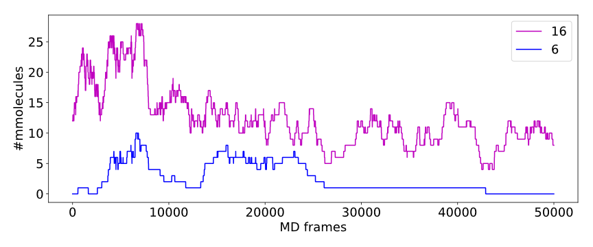
The above plot shows number of water molecules (or paths) in cluster 16 and 6 throughout the simulation. One can observe that number of molecules in cluster 6 diminishes approximately in the middle. This kind of plot can be easily generated with additional CSV data.
Number of traced paths
For each frame, numbers of traced paths are calculated for the following categories:
Name of traced molecules -
amolis used for all possible names.Paths types (
objectfor standard paths andpassingfor passing paths) -apathsis used for all possible paths types.Clusters and cluster types -
aclustsis used for all possible clusters andactypesis used for all possible cluster types.Part of paths. Possible values are:
walk,in,object,out, andin_out. Wherewalkcorresponds to any part of path and in case of passing paths only this category is used;in,object, andoutcorrespond to incoming, object, and outgoing parts;in_outcorresponds to sum of incoming and outgoing parts.
All of the above listed categories are combined together, and the final number of calculated categories may be quite big.
Size of Object and Scope
If option calculate_scope_object_size is set True and values of scope_chull and object_chull correspond to appropriate molecular entities, Aqua-Duct calculates area and volume of Scope and Object. Calculated sizes are estimated as resulting from convex hull approximations.
Visualization
Sixth stage of Valve calculations visualizes results calculated in stages 1 to 4. Visualization is done with PyMOL. Valve creates visualizations in two modes:
Two files are created: special Python script and archive with data. Python script can be simply started with python, it automatically opens PyMol and loads all data from the archive. Optionally, it can automatically save PyMol session.
PyMol is automatically started and all data is loaded directly to PyMol workspace.
Molecule is loaded as a PDB file. Other objects like Inlets clusters or paths are loaded as CGO objects.
Visualization script
By default Valve creates Python visualization script and archive with data files. This script is a regular Python script. It does not depend on AQUA-DUCT. To run it, python2.7 and PyMol are required. If no save option is used Valve saves visualization script as 6_visualize_results.py. To load full visualization call:
python 6_visualize_results.py --help

usage: 6_visualize_results.py [-h] [--save-session SESSION]
                              [--discard DISCARD] [--keep KEEP]
                              [--force-color FC] [--fast]

Aqua-Duct visualization script

optional arguments:
  -h, --help            show this help message and exit
  --save-session SESSION
                        Pymol session file name.
  --discard DISCARD     Objects to discard.
  --keep KEEP           Objects to keep.
  --force-color FC      Force specific color.
  --fast                Hides all objects while loading.
Option --save-session allows to save PyMol session file. Once visualization is loaded session is saved and PyMol closes. Option --fast increases slightly loading of objects.
Option --force-color allows to change default color of objects. It accepts list of specifications comprised of pairs ‘object name’ and ‘color name’. For example: 'scope_shape0 yellow cluster_1 blue'. This will color scope_shape0 object in yellow and cluster_1 in blue:
python 6_visualize_results.py --force-color 'scope_shape0 yellow cluster_1 blue'
Note
List of specifications has to be given in parentheses.
Note
List of specifications has to comprise of full objects’ names.
Note
Currently, --force-color does not allow to change color of molecules. It can be done in PyMol.
Options --keep and --discard allows to select specific objects for visualization. Both accept list of names comprising of full or partial object names. Option --keep instructs script to load only specified objects, whereas --discard instructs to skip specific objects. For example, to keep shapes of object and scope, as well as molecule and clusters only, one can call the following:
python 6_visualize_results.py --keep 'shape molecule cluster'
To discard all raw paths:
python 6_visualize_results.py --discard 'raw'
Options can be used simultaneously, order does matter:
If
--keepis used first, objects are not displayed if they are not on the keep list. If they are on the list, visualization script checks if they are on the discard list. If yes, objects are not displayed.If
--discardis used first, objects are not displayed if they are on the discard list and are not on the keep list.
For example, in order to display molecule, clusters, and only raw master paths, one can use the following command:
python 6_visualize_results.py --keep 'molecule cluster master' --discard 'smooth'
Note
Options --keep and --discard accepts both full and partial object names.
Note
List of names has to be given in parentheses.
Visualization objects
The following is a list of objects created in PyMOL (all of them are optional). PyMOL object names in bold text and short explanation is given.
Selected frame of the simulated system. Object name: molecule plus number of layer, if no sandwich option is used, it becomes by default molecule0.
Approximate shapes of object and scope. Objects names object_shape and scope_shape plus number of layer, if no sandwich option is used, 0 is added by default.
Inlets clusters, each cluster is a separate object. Object name: cluster_ followed by cluster annotation: outliers are annotated as out; regular clusters by ID.
List of cluster types, raw paths. Each cluster type is a separate object. Object name composed of cluster type (colon replaced by underline) plus _raw.
List of cluster types, smooth paths. Each cluster type is a separate object. Object name composed of cluster type (colon replaced by underline) plus _smooth.
All raw paths. They can be displayed as one object or separated into Incoming, Object and Outgoing part. Object name: all_raw, or all_raw_in, all_raw_obj, and all_raw_out.
All raw paths inlets arrows. Object name: all_raw_paths_io.
All smooth paths. They can be displayed as one object or separated into Incoming, Object and Outgoing part. Object name: all_smooth, or all_smooth_in, all_smooth_obj, and all_smooth_out.
All raw paths inlets arrows. Object name: all_raw_paths_io.
Raw paths displayed as separate objects or as one object with several states. Object name: raw_paths_ plus number of path or raw_paths if displayed as one object.
Smooth paths displayed as separate objects or as one object with several states. Object name: smooth_paths_ plus number of path or smooth_paths if displayed as one object.
Raw paths arrows displayed as separate objects or as one object with several states. Object name: raw_paths_io_ plus number of path or raw_paths_io if displayed as one object.
Smooth paths arrows displayed as separate objects or as one object with several states. Object name: smooth_paths_io_ plus number of path or smooth_paths_io if displayed as one object.
CoS center of the scope area (system).
CoO center of the object area (system).
Color schemes
Inlets clusters are colored automatically. Outliers are gray.
Incoming parts of paths are red, Outgoing parts are blue. Object parts in case of smooth paths are green and in case of raw paths are green if residue is precisely in the object area or yellow if it leaved object area but it is not in the Outgoing part yet. Passing paths are displayed in grey.
Arrows are colored in accordance to the colors of paths.